Compared with FTTH (fiber directly to the home), FTTB (fiber to the building) and FTTC (fiber to the curb/cabinet), FTTN keeps the fiber end point further away from the user, relies on a longer copper/coax loop, and therefore offers lower but faster-to-deploy bandwidth at a lower initial CapEx.
The focus of this article is engineering and implementation, not high-level marketing. We will look at FTTN from the perspective of planners and network engineers: standards and technologies used (VDSL2, G.fast, etc.), topology and node placement, optical and copper link budgets, cabinet and power design, deployment workflows, operations and monitoring, and how to evolve an FTTN footprint towards FTTH/FTTP over time.
Standards and Technology Stack for FTTN
From an engineering view, FTTN is a combination of fiber (PON/Ethernet) and copper (xDSL/G.fast), plus whatever local rules exist for safety, EMC and cabling.

Relevant Standards and Specifications
(1) Key ITU-T DSL / Copper Standards
ITU-T G.993.2 – VDSL2
Main standard for high-speed DSL in FTTN.
Profiles up to 17/30/35 MHz, hundreds of Mbit/s on short loops.
Defines band plans, PSD masks and performance requirements.
ITU-T G.9700 / G.9701 – G.fast
G.9700: spectrum and coexistence with legacy xDSL.
G.9701: physical layer, up to 106/212 MHz and near-gigabit rates on very short loops.
Used where the node can be placed very close to users (tens to a few hundred meters).
(2) Regional / National Standards
These don't change how FTTN "works", but they drive hardware and installation choices:
Access & cabling: mechanical, fire, UV, and in-building cabling rules.
EMC: emission/immunity limits; lightning and surge protection requirements.
Safety & grounding: earthing resistance limits, creepage/clearance, touch safety for cabinets.
Result: they mainly impact cabinet design, grounding layout, surge protection and how outside plant is built.
Copper Access Technologies in FTTN
The copper piece is what sets realistic speed and reach.
(1) ADSL2+ vs VDSL2 vs G.fast (very condensed)
ADSL2+
Up to ~2.2 MHz.
~10–20 Mbit/s over km-level loops.
Mostly legacy in an FTTN context.
VDSL2 (G.993.2)
Up to 17/30/35 MHz.
Tens to hundreds of Mbit/s on a few hundred meters.
Strongly impacted by loop length and copper quality.
G.fast (G.9700/G.9701)
Up to 106/212 MHz.
Hundreds of Mbit/s to ~1 Gbit/s on very short loops (≈50–200 m).
Needs short, clean copper (e.g., basement to apartments).
In modern builds, VDSL2 or G.fast are chosen based on how deep you can push the node into the network.
(2) Vectoring and Bonding (summary)
Vectoring
Treats all pairs in a binder like a MIMO system and cancels FEXT.
Boosts SNR and rates, especially with many active lines.
Requires that all vectored pairs are under one vectoring controller; alien lines reduce gain.
Bonding
Aggregates 2+ pairs for one subscriber.
Throughput roughly adds up if pairs are similar.
Needs similar length and quality pairs and consumes more copper per user.
In design terms: vectoring = better per-pair performance, bonding = more bandwidth per subscriber, constrained by how much "good" copper you actually have.
Interfaces to PON / Ethernet Networks
On the fiber side, an FTTN node is just an access aggregation point feeding your PON/Ethernet transport.
(1) Uplink Interfaces (Node → OLT / Aggregation)
GE / 10GE Ethernet
Point-to-point links into an aggregation switch or directly into the core.
Typical for Ethernet-centric designs.
GPON / EPON NNI
Node sits behind an OLT, connected via ONT or PON uplink module.
PON on the fiber side, DSL/G.fast on the copper side.
Choice depends on whether the network is PON-centric or Ethernet-centric, and on planned aggregation ratios.
(2) VLAN and QoS Schemes (high level)
VLANs
Per-subscriber or per-service VLANs.
Q-in-Q (802.1ad) to separate customer and provider domains.
QoS Marking
802.1p in VLAN tags for L2 priority.
DSCP in IP headers to mark traffic classes (BE, AF, EF, etc.).
Together, these let you map DSL/G.fast service profiles to differentiated treatment in aggregation/core, so voice, real-time video and critical traffic remain protected even under load.
FTTN Network Architecture and Topology Design
At a high level, an FTTN access network is a layered chain: central office → fiber (ODN) → FTTN node → copper/coax loop → CPE. The real design work is deciding where nodes sit, how many you need, and what form factor fits each area.

Typical FTTN Layered Topology
Central Office (CO) / PoP
Hosts OLTs, aggregation switches, BNG/BRAS and core routers, and connects to metro/core and the Internet. NMS/OSS systems logically sit above this layer.
ODN (Optical Distribution Network)
Fiber plant between CO and field: feeder and distribution cables, splitters, splice closures and distribution cabinets. It may be point-to-point Ethernet, GPON/EPON, or a mix, in star/tree/ring topologies.
FTTN Node (field access aggregation)
Outdoor cabinet, underground box or indoor mini-DSLAM/ DPU. Contains the DSLAM/G.fast DPU/CMTS, optical uplinks (GE/10GE or PON ONT), power and surge protection, and forms the handover point from fiber to copper/coax.
Copper / Coax Loop
Existing or new twisted-pair or coax cables from the node to subscribers or building entry points. Loop length and quality mainly determine rate and stability.
CPE (Customer Premises Equipment)
xDSL/G.fast modem, residential gateway or cable modem handling the last hop (Wi-Fi, LAN, VoIP, etc.), often auto-provisioned via TR-069 or similar.
In practice, many FTTN nodes fan out from a few COs/PoPs, with the ODN "gluing" the core to these distributed access points.
Serving Area and Node Planning Methodology
The key planning question: for a given speed target, how far from the user can the node be, and how many nodes does that imply?
(1) Loop length, target speed and service radius
Use vendor/lab speed–distance curves for the chosen xDSL/G.fast tech.
Define service profiles (e.g. ≥100/20 Mbit/s for 95% of users), then find L_max that still meets this on typical cable.
Translate L_max into a serving radius:
Theoretical: R_theoretical ≈ L_max
Practical: R_planning ≈ 0.6–0.8 × L_max to account for detours and margin.
Place nodes so all users sit within R_planning, leaving room for growth.
With G.fast, L_max can be ≤100–200 m, so nodes go to basements/curbs; with VDSL2, you usually aim for a few hundred meters.
(2) User density, geography and node count
High-density urban: many users in a small radius → fewer nodes with high fill, lower CAPEX/user, easier to justify deeper nodes and higher speeds.
Low-density suburban/rural: few users per km² → each node serves less, so you either accept longer loops/lower rates or deploy many small, lightly loaded nodes.
Geography/civil constraints (rivers, highways, hills, protected zones, existing ducts/poles) often distort the ideal circular serving areas and may force extra nodes or sub-optimal positions.
Node planning is therefore iterative: start from a radius derived from speed, overlay users and geography, then adjust locations and count to balance coverage, speed and cost.
Types of FTTN Nodes and Deployment Modes
Operators typically mix several node form factors.
(1) Outdoor cabinets
Ground-mounted roadside cabinets or pad-mounted enclosures.
Pros: high port density, ample space for power/batteries and fiber management, easy technician access.
Cons: need permits and street space, exposed to weather and vandalism, visual impact can be sensitive.
(2) Underground / wall-mounted enclosures
Underground boxes/pits: visually discreet and less exposed to vandalism, but harder to access and more at risk from water/flooding if not well sealed.
Wall-mounted boxes (facade or building entrance): shorten loops by bringing the node closer to risers; require owner agreements and suit smaller capacities.
(3) Indoor mini-DSLAMs / G.fast DPUs
Located in basements, telecom rooms or utility closets.
Pros: very short loops (ideal for high-rate VDSL2 or G.fast), controlled environment, easy building power.
Cons: need building access/agreements, limited by space and power, coordination needed for maintenance.
Real deployments usually combine larger outdoor nodes for neighborhoods with smaller indoor nodes in MDUs and business sites.
Fewer Big Nodes vs. More Small Nodes
Classic architecture trade-off:
Few large nodes further away vs many small nodes closer to users.
(1) Fewer, larger nodes
Pros: fewer sites to acquire, power and maintain; simpler backhaul; lower OPEX per node.
Cons: longer loops → lower speeds and quality; harder to deliver "near-fiber" performance; less flexible when hotspots need much higher bandwidth.
(2) More, smaller nodes
Pros: shorter loops → higher rates and stability; better targeting of high-value areas; smoother evolution path towards FTTC/FTTB/FTTH with reusable deep nodes.
Cons: more sites, more uplinks, more civil works and coordination; higher initial complexity and cost.
In practice, you look for a sweet spot: enough nodes to meet service-level objectives on loop length and speed, but not so many that site, power and backhaul costs become unmanageable.
Physical Layer & Outside Plant Engineering
At the physical layer, an FTTN network is a fiber ODN feeding a cabinet, and from there a bundle of copper or coax loops fan out to users. Whether the solution works well in real life is largely decided here: link budgets, cable types, loop lengths and binder management.

Fiber Side: ODN Structure and Optical Link Budget
ODN hierarchy in an FTTN context
A typical ODN (Optical Distribution Network) for FTTN looks like this:
CO ODF (Central Office Optical Distribution Frame)
Termination for feeder/trunk fibers leaving the central office or PoP.
Cross-connect to OLT or aggregation switches (via SFP/SFP+ ports).
Trunk / Feeder Cable
High-fiber-count cable running out of the CO along primary routes (ducts, poles).
Often 24F, 48F, 96F or larger, depending on how many FTTN nodes and other access points it must serve.
Splitters / Splice Closures
For PON: 1:N splitters (e.g., 1:8, 1:16, 1:32) in splice closures or dedicated splitter cabinets.
For point-to-point Ethernet: just splices and distribution/aggregation points, no splitters.
Distribution Cabinet / Fiber Distribution Point
Fan-out from trunk fibers (or PON splitters) to individual FTTN nodes.
Provides patching, splicing, and some margin for future growth.
FTTN Node Fiber Termination
At the node, fibers terminate on patch panels, then jumpers go to the DSLAM / DPU / uplink optics.
This is the endpoint of the ODN in an FTTN scenario.
The ODN must be designed such that optical loss from CO to any FTTN node stays within the optical budget for the chosen PON class or Ethernet optics.
Link budget basics
The basic inequality for any optical link is:
P_tx – Total Loss ≥ P_rx_min + Margin
Where:
P_tx = transmit power of the optical port (dBm)
Total Loss = sum of all losses along the path (dB)
Fiber attenuation (dB/km × distance)
Connector losses (dB per connector)
Splice losses (dB per splice)
Splitter losses (for PON, dB depending on split ratio)
P_rx_min = minimum receiver sensitivity (dBm) for correct operation
Margin = design margin (typically 2–5 dB) for aging, repairs, temperature, small measurement errors, and future changes.
If this inequality is not satisfied, you either need to shorten the path, reduce losses, use a different optics class, or relax the split ratio.
Example link budget for a PON-based FTTN ODN
This is a simplified example, just to illustrate the calculation.
Assume:
GPON OLT, Class B+ optics
P_tx ≈ +3 dBm
P_rx_min ≈ –27 dBm
Feeder+distribution fiber length: 10 km
Attenuation: 0.35 dB/km (1310 nm) → 10 × 0.35 = 3.5 dB
Connectors: 4 connectors total (at OLT, ODF, cabinet, node)
0.5 dB per connector → 4 × 0.5 = 2 dB
Splices: 10 splices total along the route
0.1 dB per splice → 10 × 0.1 = 1 dB
Splitter: 1×32 PON splitter
Insertion loss ≈ 16.5 dB
Design margin: target 3 dB
Now compute:
Total Loss (without margin) = 3.5 + 2 + 1 + 16.5 = 23 dB
Available power budget = P_tx – P_rx_min = 3 – (–27) = 30 dB
Check the inequality including margin:
Left side: P_tx – Total Loss = 3 – 23 = –20 dBm
Right side: P_rx_min + Margin = –27 + 3 = –24 dBm
Result: –20 dBm ≥ –24 dBm → OK, with 4 dB of effective margin.
In an FTTN deployment, fiber distances are often shorter than typical FTTH PON distances, so ODN design is usually more forgiving, but this budget must still be checked for every planned node.
Copper Side: Loop Characteristics and Cable Selection
Once you leave the FTTN node, the copper loop is the main bottleneck. Its electrical characteristics directly affect attenuation, SNR and hence achievable bit rate.
Resistance, capacitance, attenuation vs conductor size
Typical twisted-pair telecom cables might use conductor diameters like:
0.4 mm (roughly 26 AWG)
0.5 mm (roughly 24 AWG)
0.6 mm (roughly 22 AWG)
In general:
Smaller diameter → higher resistance, higher attenuation per km.
Larger diameter → lower resistance, lower attenuation, better performance at longer loops.
Attenuation is also frequency-dependent: higher frequencies (used by VDSL2/G.fast) suffer higher loss per km. For a rough sense (planning-level only, actual numbers depend on cable type and frequency):
0.4 mm pair: higher attenuation per km → loops should be shorter for high-speed profiles.
0.5 mm pair: common compromise in many access networks.
0.6 mm pair: better long-distance performance, but more expensive and heavier.
Vendors usually provide attenuation vs frequency vs distance curves. During planning, you select the worst-case cable type and frequency that your DSL profile will use, and then derive maximum loop lengths.
Distance vs achievable data rate (example)
For illustration, consider VDSL2 profile 17a on reasonably good 0.5 mm twisted pair, with vectoring enabled and no severe noise sources. A very simplified, indicative table might look like:
| Loop length (approx.) | Typical downstream rate (indicative) |
|---|---|
| 300 m | 100–130 Mbit/s |
| 500 m | 80–100 Mbit/s |
| 800 m | 50–70 Mbit/s |
Important notes:
These are ballpark planning figures, not guaranteed rates.
Real performance depends on:
Cable type and condition
Binder fill and crosstalk
Noise margin settings
Vectoring effectiveness
Vendors will usually give more precise curves (with and without vectoring, with specific SNR margin, etc.).
For G.fast, think of much shorter loops and higher data rates, e.g.:
50–100 m: several hundred Mbit/s up to around 1 Gbit/s (depending on profile, spectrum, vectoring).
100–200 m: noticeably lower but still very high rates compared to VDSL2.
This is why G.fast deployments often push equipment into basements or very close to the building.
Crosstalk in binder groups and binder management
In multi-pair cables, pairs are grouped in binders. Crosstalk between pairs is one of the dominant degradation mechanisms:
NEXT (Near-End Crosstalk)
Interference from a transmitter into a receiver at the same end of the cable.
More critical for full-duplex or overlapping frequency schemes.
FEXT (Far-End Crosstalk)
Interference from a transmitter at one end into a receiver at the opposite end.
A major limitation for VDSL2 and G.fast, especially as more lines in the binder are active.
Engineering responses:
Keep binder organization consistent: group lines with similar technology and service profile together.
Avoid mixing different DSL profiles or bit-loading schemes in the same binder when possible.
Coordinate with other operators (if unbundled) so "alien" lines don't destroy crosstalk assumptions.
Good binder management reduces variance and allows vectoring algorithms to work more effectively.
Engineering Aspects of Vectoring and Bonding
Vectoring requirements
Vectoring attempts to cancel FEXT by treating all lines in a binder as one big multi-pair system. For it to work in practice:
All vectored lines must be terminated on the same vectoring engine
Usually means all lines in the vectoring group are on the same DSLAM or the same set of line cards that share a vectoring unit.
Binder composition must be known and controlled
Adding a new non-vectored line in the same binder can introduce uncontrolled interference.
In unbundled environments (multiple operators in the same cable), full vectoring may not be achievable.
Line conditions should be reasonably stationary
Frequent connect/disconnect in the binder complicates vectoring calibration.
Sudden loop changes (repairs, re-termination) may temporarily hurt performance until recalibration.
From an FTTN design point of view, this means you want:
Clean binder allocation for vectored groups.
As much single-operator control as possible over those binders.
Node capacity sized such that "orphan" non-vectored lines are minimized.
Bonding sensitivity to loop symmetry
Bonding aggregates multiple copper pairs for one subscriber (e.g., dual-pair VDSL2). For bonding to work well:
Loop lengths must be similar
Large differences in length cause different propagation delays and attenuation per pair.
The overall throughput is often limited by the weakest pair.
Loop quality should be consistent
One heavily degraded pair can drag down the bonded link.
It may be better to keep one good single pair than bond it with a very poor one.
Outside plant routing
Ideally, bonded pairs follow the same physical path (same cable, same binder) to keep environmental impacts similar.
Mixing pairs from different cables or very different routes increases asymmetry.
Practically, this means the outside plant engineer must:
Reserve and document pair groups intended for bonding.
Make sure they run together through the same closures and cabinets.
Reflect any changes (repairs, reroutes) in records, so operations teams know when a bonded line might have become unbalanced.
Bandwidth Planning and Performance Modeling
FTTN bandwidth planning is essentially answering three questions:
What do users want to do? (applications)
What speed do I need to deliver that with margin? (per-subscriber bandwidth)
How many subscribers can I safely multiplex on uplinks and core links? (oversubscription & QoS)

From Applications to Speed and Loop Constraints
You start with a service mix, not with a random Mbps number.
Typical household / SME service mix example
For a modern home or small office, realistic concurrent demand might look like:
1–2 × 4K video streams (OTT / IPTV)
1–3 × HD video calls (Teams/Zoom)
Several always-on cloud apps (Office 365, web browsing, SaaS tools)
Background traffic: OS updates, backups, IoT, smart cameras, etc.
Back-of-the-envelope dimensioning per household might be:
- 4K stream: ~20–25 Mbit/s (with some overhead)
- HD video call: ~2–3 Mbit/s
- "Everything else": say 5–10 Mbit/s of headroom
So for a "demanding" household:
- Peak downstream: 2×25 + 3×3 + 10 ≈ 80–90 Mbit/s
- Peak upstream: dominated by video calls + cloud sync, say 10–20 Mbit/s
- Operators typically round up and market tiers like 100/20 Mbit/s, 200/50 Mbit/s, etc., to build in margin and simplify product portfolios.
From speed to loop constraints
Once you decide a tier (e.g., 100/20 Mbit/s):
- Look at VDSL2 / G.fast speed–distance curves (vendor or lab data).
- Find the maximum loop length L_max where your tier can be delivered with a comfortable noise margin (e.g., 6 dB).
For planning, derate that a bit (e.g., use 80–90% of L_max) to account for:
- Cable quality variations
- Crosstalk when many lines are active
- Ageing and repairs
If the service tier is non-negotiable, L_max becomes a hard constraint on node placement. If node placement is constrained (few sites allowed), the tier may need to be less ambitious for users far from the cabinet.
Port Capacity and Oversubscription Design
Per-subscriber bandwidth is not the same as what you must provision on uplinks. In practice, users are bursty and not everyone is at peak at the same time, so you can oversubscribe.
(1) Oversubscription across layers
Three main layers:
Access: DSL/G.fast ports on the FTTN node → uplink(s)
Aggregation: multiple FTTN nodes → aggregation switches / rings
Core / edge: aggregation → BNG/BRAS and Internet peering
The principle is:
The closer to the user, the lower the oversubscription ratio (more conservative).
The closer to the core, the higher the ratio you can tolerate (because of statistical multiplexing across many users).
(2) Example oversubscription ratios
These are not rules, but commonly used starting points:
Residential best-effort users
Access uplink: 1:4 to 1:8
E.g., 100 × 100 Mbit/s ports (10 Gbit/s "contracted") → 1–2.5 Gbit/s uplink.
Aggregation / core: 1:8 to 1:20, depending on service commitments.
SMB / prosumer users
Access uplink: 1:2 to 1:4
Aggregation / core: typically lower ratios if they have "business" SLAs.
Enterprise / dedicated access
Often no oversubscription on specific paths (or very low, e.g. 1:1–1:2), especially for guaranteed bandwidth services.
When setting these ratios, consider:
How many users share each node and each uplink.
Time-of-day traffic profiles (prime time vs business hours).
Competitive pressure: if you're in a market with aggressive claims ("no slowdowns at peak"), you must dimension more generously.
Oversubscription planning is typically done with traffic models or historical statistics, but for new builds you start with conservative ratios and adjust as real data arrives.
QoS and Latency Performance
Throughput is only half the story; delay and jitter determine whether real-time services feel "snappy" or "laggy".
(1) Queuing, buffering and their impact
Every node (DSLAM, aggregation switch, router) has queues and buffers:
- Under light load, packets pass with minimal queuing delay (microseconds to small milliseconds).
- Under congestion, queues fill and buffering adds tens to hundreds of milliseconds of delay.
- Poor buffer management can also cause bufferbloat, where large queues get filled by bulk traffic and delay all flows.
In FTTN networks you want:
Reasonable buffer sizes: enough to smooth small bursts but not so big that they create huge delays.
Proper queueing disciplines (e.g., priority queues or weighted fair queuing) so that real-time traffic doesn't sit behind large downloads.
(2) Practical latency and jitter targets
Common engineering guidelines (one-way, access + aggregation, not including distant Internet paths):
VoIP / voice
One-way latency: ideally < 50–80 ms inside the operator network.
Jitter (variation): keep < 20–30 ms; use jitter buffer in endpoints.
Packet loss: well below 1%.
Interactive video (video conferencing)
Similar to VoIP, but a bit more tolerant to jitter due to larger playout buffers.
Aim for one-way < 100 ms inside your domain; end-to-end with Internet typically higher, but keep access/aggregation contribution small.
Cloud gaming / real-time interactive apps
Very sensitive to latency and jitter.
Target round-trip within your network (CPE ↔ edge/border) in the < 20–30 ms range if possible.
Use QoS to prioritize gaming packets over bulk transfers when congestion occurs.
(3) Mapping QoS classes
To achieve these targets over an oversubscribed network:
Classify traffic at the FTTN node / CPE:
Voice / gaming / real-time → high priority queues.
Video streaming → medium priority with sufficient bandwidth.
Bulk downloads, backups, updates → best-effort queues.
Mark packets with 802.1p / DSCP and keep those markings consistently respected through aggregation and core.
Dimension queues and link capacities such that high-priority classes almost never hit sustained congestion, or at least have guaranteed minimum bandwidth.
Deployment and Turn-Up Process
From a project view, FTTN rollout is a pipeline: survey → build → install → configure → test → accept. Quality here decides how much trouble you have later in O&M.

Site Survey & High-Level Planning
(1) Route survey & environment
Check planned routes and node locations.
Record: existing ducts/manholes/poles, space for cabinets/boxes, obstacles (roads, rivers, rail, private land).
Verify nearby power: availability, capacity, metering option.
(2) Copper plant inventory
Identify cable types, pair counts, binder structure, age, known problem segments.
Note existing cross-connects and typical loop lengths.
Do sample pair tests (resistance, insulation, simple TDR) to confirm if copper can support VDSL2/G.fast.
Output: high-level design with proposed node sites, serving areas, main fiber/copper routes, first-pass BOM.
ODN Construction
(1) Fiber cable laying
Install feeder/distribution fiber in ducts or on poles.
Respect bend radius, pulling tension and properly seal ducts/closures.
(2) Splicing & termination
Splice according to ODN plan (feeder → distribution → node).
Use labeled splice trays and terminate at CO ODF and node patch panels.
(3) OTDR & power-level tests
OTDR new spans to confirm total loss and locate bad splices/bends.
Measure received power at nodes vs link budget and archive results as as-built data.
Node Installation and Wiring
(1) Cabinet / enclosure
Install on pads/brackets with enough clearance and mechanical stability.
(2) Grounding & power
Connect to earthing system and verify ground resistance.
Install/test power (AC/DC, –48 V, breakers, surge protectors, optional batteries).
(3) Internal wiring
Mount DSLAM/G.fast DPU and auxiliaries.
Patch fibers to uplink ports.
Jumper copper pairs to line cards per serving plan with clean labeling and cable management.
Configuration and Testing
(1) DSLAM/OLT configuration
Basic setup: management IP, routing, SNMP/Netconf, NTP, syslog.
Uplinks: VLANs/Q-in-Q, LAG if needed.
Access: line profiles (rate, vectoring, SNR margin, INP, interleaving), assigned per port/plan.
QoS: map VLANs to classes and shaping/policing per product tier.
(2) Uplink & loop testing
Uplink: verify reachability, routing and run throughput checks.
Lines: check sync rate, SNR margin, attenuation, CRC/FEC; use built-in loop diagnostics if available.
Problem lines (low SNR, high errors, low sync) are flagged for copper plant fixes.
Trial Run and Acceptance
(1) KPIs during pilot (e.g., 2–4 weeks)
- Bandwidth: throughput vs product tier, peak-hour utilization on uplinks.
- Packet loss: in operator domain, watching for bursty loss.
- Latency/jitter: access + aggregation share; validate VoIP, video, gaming behavior.
- Stability: re-sync counts, error bursts, power/cabinet alarms.
(2) Acceptance
Define thresholds (min sync rate, max failure rate, latency budget).
If KPIs and pilot user feedback are OK, hand over to operations and start full rollout.
Operations, Monitoring and Maintenance
In production, FTTN becomes mainly an operations challenge: keep performance stable, faults rare, and troubleshooting fast.

Performance Monitoring and Alarms
(1) Device-level
Monitor temperature, PSU/fan/battery, input voltage, power failures.
Track uplink port status and line card health.
Feed all into NMS with clear severity and correlation rules.
(2) Line-level
For each xDSL/G.fast line: SNR margin, attenuation, CRC/HEC, FEC, SES, UAS.
Use trends over weeks/months to spot aging copper, water ingress, rising interference.
Dynamic Line Management (DLM)
DLM auto-tunes line parameters based on error stats:
Inputs: CRC/FEC rates, re-syncs, SNR margin trends.
Actions: lower max rate, raise target margin, change interleaving/INP.
Goal: fewer errors and drops, even at slightly reduced peak speed.
For most residential users, stability > headline rate.
For SLA lines, DLM policies may be stricter or partially manual.
NOC must see when/where DLM changed profiles and be able to tune policies over time.
Fault-Location Methodology
Use a layered, structured approach instead of random guessing:
CPE / premises
Check power, Wi-Fi, LAN, user equipment.
Compare with other users on the same node.
Copper loop
Run line tests for HR joints, shorts/opens, bridged taps, abnormal attenuation.
Typical causes: moisture, old insulation, animal damage, poor splices.
FTTN node
Check port and card status, alarms, power/temperature.
Fiber / ODN
Check uplink errors/flaps/LOS; use OTDR if fiber damage is suspected.
CO / upstream
Validate aggregation/BNG/router health, routing/QoS changes.
Keep a "top suspects" list: water ingress, aging pairs, power issues, and bad configs/software pushes causing wide-area incidents.
Remote OAM and Automation
Modern FTTN needs remote control + automation, not per-box manual work.
(1) Frameworks
TR-069 / TR-369 for CPE config, diagnostics and firmware.
SNMP / Netconf/YANG / REST for nodes and aggregation gear.
Syslog / telemetry for central log and KPI collection.
(2) Automation
Provisioning: template-based configs, auto-assign profiles from orders.
Upgrades: staged, scheduled software rollout with rollback and version tracking.
Alarm correlation: power + temperature + port/line alarms combined to point at root cause (e.g., single fiber cut vs many DSL issues).
Done well, this cuts OPEX and MTTR and makes FTTN a predictable, low-drama part of the access network instead of a constant firefight.
Engineer-Focused FAQ

Max loop length for typical speeds?
~50–80 Mbit/s: ≈ 700–900 m (VDSL2 + vectoring, 0.5 mm).
~100 Mbit/s: ≈ 400–600 m.
≥200 Mbit/s: ≤300 m or go G.fast (≤100–200 m).
→ Always use vendor curves and derate ~20–30%.
Pair count / binder composition impact?
More active pairs + mixed technologies in one binder → more crosstalk → lower SNR and real rates.
Best case: all pairs same operator + same tech + vectoring group.
Can legacy ADSL copper keep working for FTTN?
Do sample tests: resistance, insulation, TDR + multi-day VDSL2/G.fast trials (SNR, CRC/FEC, SES/UAS).
Isolated issues → local rehab; widespread issues → cable rehab or more/deeper nodes.
What's reusable when moving to FTTH?
Usually reusable: CO/PoP, ducts, poles, most feeder/distribution fiber, power/ground at sites.
Mostly replaced: copper loops, DSLAM/DPUs (and sometimes old cabinets).
Plan FTTN so ODN/sites are FTTH-ready.
How to balance node count vs user experience under tight CapEx?
Deeper/more nodes for high-density/high-ARPU zones; longer loops/lower tiers for low-value areas.
Compare simple scenarios on "CapEx per Mbps delivered" and meet SLA with minimum total cost, not minimum sites.
How to keep O&M cost under control?
Central NMS + a small KPI set (SNR, CRC/FEC, SES/UAS, ports, temp, power) + strong automation (templates, TR-069, Netconf/REST).
Target: early detection + remote fixes, minimal truck rolls.