A 1×16 PLC splitter can fit a local FTTH distribution point, but "sixteen outputs" is not enough to approve the design. The planner must know whether the 1×16 device is the only splitter in the optical path or one stage in a cascaded PON, because that changes the effective total split, optical loss, fault-isolation points, enclosure layout, port records, and future activation workflow.
This guide focuses on that narrow engineering task: deciding whether a 1×16 PLC splitter belongs at a distributed or second-stage FTTH node, then defining the loss budget, output map, physical integration, acceptance tests, and RFQ fields around it. For general PLC splitter types, packages, and ratio selection, use the PLC splitter guide.
Define "Distributed" on the Network Drawing First
Do not approve a 1×16 splitter from the word "distributed" alone. Depending on the network convention, the term may describe a splitter moved deeper into the access network or a design with multiple cascaded split locations. The drawing should therefore show every split stage explicitly.
For the serving area that contains the 1×16 device, record:
- the OLT/PON port or upstream feeder that supplies the node;
- every upstream splitter and its ratio;
- the location and role of the 1×16 splitter;
- the sixteen downstream output identifiers;
- the subscriber/drop area served by those outputs;
- connectors, splices, adapters, and other passive events between stages;
- planned spare outputs and how they will be protected and documented.
If there is no upstream optical split, the local 1×16 represents an effective 1:16 split. If a first-stage splitter already exists, the total split is the product of the stages. That distinction must be settled before the optical budget or subscriber count is evaluated.

Calculate the Effective Total Split Before Checking Capacity
For balanced splitters in cascade, multiply the ratios along one optical path. A 1×4 first stage feeding a 1×16 local splitter does not remain a "1×16 PON"; the effective split from the original input to the final outputs is 1×64.
The theoretical equal-power splitting loss is a useful sanity check:
Ideal splitting loss = 10 × log10(N), where N is the effective number of equal output paths.
| Splitter path | Effective total split | Ideal equal-split loss floor | Planning note |
|---|---|---|---|
| 1×16 only | 1×16 | About 12.04 dB | Single split stage. |
| 1×2 → 1×16 | 1×32 | About 15.05 dB | Two split locations; check both splitter specifications and the interstage path. |
| 1×4 → 1×16 | 1×64 | About 18.06 dB | Higher total split; verify that the selected PON equipment and complete ODN budget support it. |
| 1×8 → 1×16 | 1×128 | About 21.07 dB | Mathematical example only, not an approval recommendation; architecture or optical budget may rule it out. |
The Fiber Optic Association's splitter testing reference shows the same basic physics: each factor-of-two split adds roughly 3 dB of ideal splitting loss. Cisco's PON cabling and power-budget reference likewise separates theoretical splitting loss from other splitter loss terms.
Do not use the ideal values in this table as product acceptance limits. Real splitter insertion loss is higher than the theoretical split floor because the complete device has additional loss. The selected splitter datasheet and project specification must supply the actual design and acceptance values.

Budget a Cascaded 1×16 Path Without Double-Counting Splitter Loss
The safest budget starts with the exact active equipment and the exact passive path. Use the approved OLT/ONT optical budget or platform design limit, then subtract the maximum planned losses of the ODN.
A practical planning equation is:
Planned ODN loss = fiber loss + connector-pair loss + splice loss + upstream-splitter maximum insertion loss + 1×16 maximum insertion loss + other passive losses
Then evaluate the remaining margin using the project's approved engineering method.
One error is especially important to avoid: if a splitter datasheet already gives maximum insertion loss for the complete splitter, do not add the theoretical 10 × log10(N) value again. The theoretical value is a physics check; the datasheet insertion-loss value is the component value used in the design budget when the specification defines it that way.
| Budget item | Value source | What to verify |
|---|---|---|
| Active-system optical budget | Approved OLT/ONT or platform documentation | Correct PON technology, optical class/profile, wavelength direction, and project limits. |
| Upstream splitter stage | Approved splitter datasheet or project specification | Exact ratio, termination, maximum insertion loss, and applicable test condition. |
| Local 1×16 splitter | Approved 1×16 datasheet or purchase specification | Maximum insertion loss and any required uniformity, return-loss, or PDL criteria. |
| Interstage and drop fiber | Approved cable data and route length | Design wavelength and installed length. |
| Connectors and splices | Project design values and actual connection count | Count every planned event; do not hide extra adapters or repair joints. |
| Engineering reserve | Operator/project rule | Use the approved margin policy rather than a generic internet value. |
If you need to build the complete link worksheet, use DIMI's fiber loss and power-budget guide. The calculation here focuses on the cascade-specific contribution of the upstream stage and local 1×16 splitter.

When a Local 1×16 Node Makes Operational Sense
A local 1×16 splitter is most defensible when sixteen output positions form a useful service group at that location and the complete PON remains inside its approved architecture and optical budget. The engineering question is not whether sixteen customers exist somewhere in the project; it is whether those sixteen output paths belong at the same access node.
Check the following together:
- Service-area density: the local cluster should justify up to sixteen output positions without creating excessive drop routing.
- Upstream split: any earlier splitter stage must be included in the effective total ratio and loss budget.
- Take rate and growth: decide how many outputs are active at launch and which outputs remain protected spares.
- Enclosure capacity: the box or closure must accommodate the splitter body, leads, adapters or splices, bend control, labels, and future access in the populated state.
- Fault isolation: technicians must be able to distinguish a common upstream fault from a single output/drop fault.
- Restoration: the design should identify which components are replaceable and how a failed splitter or damaged output lead is accessed.
A 1×16 node is a weak choice when it forces an unsupported total split, consumes too much optical margin, creates long or awkward downstream drops, cannot be serviced inside the intended enclosure, or leaves the operator with poor records across multiple split locations.
Keep Package Selection Separate From Split-Ratio Approval
The optical ratio does not tell you whether the 1×16 device should be blockless, ABS, cassette, rack-mounted, bare-fiber, connectorized, or spliced. That decision belongs to the physical installation point.
Confirm:
- available enclosure volume and mounting method;
- connectorized versus fusion-spliced input/output interfaces;
- connector family and polish when connectors are used;
- fiber/pigtail construction and lead length;
- minimum routing space and service loops defined by the approved components;
- how the splitter is retained so leads are not carrying mechanical load;
- whether a technician can replace or test the splitter without disturbing unrelated fibers.
For a detailed physical-format comparison, use Blockless vs Cassette PLC Splitters. The 1×16 architecture should be approved first; package selection then implements that architecture at the chosen node.
Map All 16 Outputs Before Installation
A distributed node becomes difficult to operate when the splitter outputs exist physically but are not tied to a controlled service map. Numbering should be consistent across the splitter, adapters or splice tray, drop cable labels, outside-plant records, and subscriber records.
| Record field | What it should identify |
|---|---|
| Splitter ID | Unique node/splitter identifier tied to the location. |
| Input source | Feeder fiber and, where applicable, upstream splitter output. |
| Output 01–16 | Assigned drop, terminal port, address, or reserved status. |
| Physical termination | Adapter number, splice position, or connectorized output. |
| Activation state | Active, reserved, spare, unavailable, or other operator-defined status. |
| Test record | Reference to the applicable incoming or installed optical result. |
Unused outputs should remain protected according to the connector or enclosure instructions and should still appear in the record. A spare port that is uncapped, unlabeled, or absent from the map is not a controlled growth resource.
Accept the 1×16 Node as a System, Not Just a Splitter Part Number
Acceptance should prove identity, optical behavior, mapping, cleanliness, and installed serviceability. The exact test procedure and pass/fail limits must come from the project specification and the approved splitter data.
- Verify identity. Match ratio, package, input/output termination, lead configuration, labels, and drawing revision to the approved order.
- Verify the cascade. Confirm the actual upstream stage and calculate the installed effective total split. Do not allow an undocumented extra splitter stage.
- Inspect optical interfaces. For connectorized assemblies, inspect, clean when required, and re-inspect before mating.
- Verify the 16-output map. Confirm each output reaches the intended adapter, splice, terminal, or drop record.
- Measure the required optical paths. Where full-port acceptance is required, test all sixteen outputs; where a sampling plan is permitted, define it explicitly. Compare results with the approved product/project limits rather than a generic internet value.
- Check channel variation where specified. Excessive port-to-port variation can indicate a component, connector, splice, contamination, or test-reference problem; use the approved uniformity criterion if the project defines one.
- Verify the complete ODN path. Confirm that the final link remains within the approved optical budget after both splitter stages and all other passive events are included.
- Save the as-built record. Preserve splitter IDs, upstream/downstream mapping, test files, active/spare outputs, enclosure location, and drawing revision.

Troubleshoot by the Failure Pattern
| Observed condition | Check first | Reasoning |
|---|---|---|
| All 16 outputs are unavailable | Input fiber, upstream splitter/output, common connector/splice, and local splitter input | A common-path fault can affect every local output at once. |
| All outputs show less margin than expected | Budget assumptions, undocumented split stage, common-path contamination/loss, and splitter identity | A shared design or upstream loss error is more likely than sixteen independent drop faults. |
| One output is abnormal | That output lead/connector/splice, drop fiber, and subscriber-side termination | A single-channel problem should be isolated before changing the common splitter path. |
| Several subscriber records are wrong but optics are normal | Port map, labels, adapter numbering, and as-built database | Continuity can be correct while subscriber assignment is wrong. |
| A spare fails when first activated | Protection cap, connector cleanliness, record accuracy, unused adapter, and downstream drop | Long-unused interfaces need the same inspection discipline as active ports. |
In a multi-stage PON, troubleshooting requires records at more than one splitter location. That is one of the operational costs of a cascaded architecture, so the design should make test boundaries and common-path relationships visible before service is activated.
What to Put in a 1×16 PLC Splitter RFQ
When comparing a 1×16 PLC splitter supplier, the quotation should describe the actual node rather than only the phrase "1×16 PLC splitter." Supplier comparison should follow the engineering definition of the node, not replace it.
- network role: single-stage local split or second-stage/cascaded split;
- upstream splitter ratio, if any, and effective total split;
- approved PON/platform context and project optical-budget reference;
- splitter package and mounting requirement;
- input/output termination: splice or connectorized;
- connector type and polish where applicable;
- fiber/pigtail type, length, and identification requirement;
- maximum insertion loss from the approved product specification;
- uniformity, return loss, PDL, wavelength, or other optical criteria when the project requires them;
- output numbering 01–16 and label format;
- enclosure/adapter/splice integration drawing;
- required incoming test report or per-port data;
- packaging and end-face protection requirements;
- drawing revision and change-notification requirement.
For commercial configurations and quotation, use the DIMI PLC Splitter category. Do not copy unverified website performance values into the project specification; require the approved datasheet or project document for the exact quoted construction.
Final Design Rule
A 1×16 PLC splitter is justified by the complete ODN, not by its port count. Draw every split stage, multiply cascaded ratios, use theoretical splitting loss only as a sanity check, budget the real splitter stages with approved maximum insertion-loss values, and map all sixteen outputs before installation. Once the optical budget, local service area, enclosure, testing method, and operating records agree, the 1×16 node becomes a controlled part of the FTTH architecture rather than an isolated catalog item.
FAQ
Q: Is a 1×16 PLC splitter always a second-stage splitter?
A: No. It can be used as a single split stage or as one stage in a cascaded design. The network drawing must show its actual role.
Q: If a 1×4 splitter feeds a 1×16 splitter, what is the total split?
A: The effective split is 1×64. The ideal equal-split loss floor is about 18.06 dB, but the design budget must use the approved maximum insertion loss of each real splitter plus fiber, connectors, splices, and other passive losses.
Q: How much loss does a 1×16 splitter add?
A: The theoretical equal-power split alone is about 12.04 dB. Actual insertion loss is higher and varies by product construction and termination, so use the approved datasheet value for the exact splitter rather than treating 12.04 dB as an acceptance specification.
Q: Can unused 1×16 outputs be kept for future growth?
A: Yes, if the network plan allows it. Keep unused interfaces protected, labeled, included in the port map, and accessible without disturbing active fibers.
Q: Should I choose 1×16 or 1×32?
A: Start with the required total split, active-system support, optical budget, service-area density, and maintenance model. If 1×32 is being evaluated as the primary ratio, use DIMI's 1×32 PLC splitter selection guide for the ratio-specific checks.