A 100G spine-leaf fabric is one of the most dependable ways to connect 25G servers, 100G uplinks, storage clusters, and east-west-heavy workloads in a modern data center. The appeal of QSFP28 is its flexibility: a single port can carry a native 100G link or break out into four 25G server connections, so one switch can serve both the access edge and the fabric core.
Fast switches are the easy part. A 100G design lives or dies on the decisions made before the purchase order: how each port is allocated, what the oversubscription ratio looks like under normal and failure conditions, which optics match the real cable runs, how much heat those optics add, and whether the fabric can grow toward 400G without a forklift upgrade.
This guide is a vendor-neutral planning reference for network and infrastructure teams. The figures below follow current IEEE 802.3 Ethernet specifications and the relevant optical multi-source agreements, but every switch and transceiver has its own datasheet, so confirm the exact numbers for the hardware you buy.
How to read the examples in this guide. Unless stated otherwise, they assume single-homed servers with one 25G NIC each, 48 host ports per leaf, 100G leaf-to-spine uplinks, a full mesh in which every leaf connects to every spine, and forward error correction enabled where the optics require it. Dual-homing, faster NICs, or different port counts will change every number that follows.
What Is a 100G Spine-Leaf Network?
Spine-leaf is a two-tier data center architecture built from leaf switches and spine switches. Leaf switches sit at the top of each rack and provide server-facing ports plus uplinks to the spine. Spine switches form the high-speed backbone. Every leaf connects to every spine, so traffic between racks moves leaf to spine to leaf along an equal-length path.
The design is popular because it delivers:
- Predictable, equal path length between any two racks
- Native support for heavy east-west traffic
- All uplinks active through ECMP rather than blocked by spanning tree
- Simple horizontal scaling - add leaves for ports, add spines for capacity
In a 100G fabric, leaf-to-spine links run at 100G, while server-facing ports run at 10G, 25G, 50G, or 100G depending on the workload. Today, 25G access with 100G uplinks is the most common enterprise combination.

Physical Design vs Logical Design
"Network design" covers two layers that are easy to conflate. This guide concentrates on the physical and capacity layer - ports, optics, oversubscription, cabling - because that is what you commit to when you buy hardware. But the logical layer decides how the fabric forwards traffic, and it shapes several physical choices.
On the physical side sit switch and port selection, NIC speeds, oversubscription, optics, cabling, power, and cooling. On the logical side sit ECMP load-balancing across uplinks; an overlay such as VXLAN with a BGP EVPN control plane for multi-tenant Layer 2 and Layer 3 over a routed underlay; dual-homing with MLAG or MC-LAG and LACP at the access edge; and failure-domain sizing. For RDMA fabrics you also have to engineer a near-lossless network, covered below. Settle the logical model early, because it affects uplink counts, how many spines you want for ECMP width, and whether leaves are deployed as MLAG pairs.
Step 1 - Define Server Speed and Workload
Start with the workload, not the optics. A general virtualization cluster, a storage fabric, and an AI training pod have very different needs, and the right design follows the traffic.
25G servers with 100G uplinks
For most enterprise and private-cloud environments, 25G access with 100G leaf-to-spine uplinks is the sweet spot: a large jump over 10G while keeping NIC, cable, and switch costs reasonable. A typical build pairs 25G downlinks, 100G uplinks, and a 2:1 to 3:1 ratio for general compute, with lower oversubscription reserved for storage and latency-sensitive tiers. It fits virtualization, private cloud, web tiers, and the bulk of enterprise data centers.
Native 100G for storage, AI, and HPC
Some workloads need native 100G to the server: distributed and NVMe-oF storage, AI and machine-learning training, HPC, large-scale analytics, and low-latency RDMA. Here oversubscription should be low - often non-blocking or close to it - because the traffic pattern is the problem, not just the volume.
AI, HPC, and RDMA workloads generate dense, synchronized, all-to-all east-west traffic: many nodes transmit to many nodes at the same moment, so the statistical smoothing that saves you on a virtualization fabric no longer applies. RDMA over Converged Ethernet (RoCE) adds a second constraint, because it expects a near-lossless fabric, which in practice means Priority Flow Control (PFC) and Explicit Congestion Notification (ECN) tuned end to end. A fabric that drops frames under congestion will watch RoCE performance collapse, so these clusters are usually built at 1:1 with careful buffer and congestion configuration.
Step 2 - How to Calculate Leaf and Spine Switch Ports for a 100G Fabric
Port planning starts at the leaf, not the spine. Work outward from the servers:
- Count server-facing ports per rack.
- Decide whether each is native 25G, native 100G, or a breakout lane.
- Reserve QSFP28 ports for spine uplinks.
- Add spare ports for growth, redundancy, test, and replacement.
- Recalculate oversubscription after breakout is assigned, not before.
Count server-facing ports
For each rack, pin down server count, NIC speed, NICs per server, single- or dual-homed, and required spares. A rack of 48 servers with one 25G NIC each needs 48 host ports. Dual-home those servers to a leaf pair and the access port count across the pair doubles.
Reserve uplink ports, and watch the double-count
After host ports, reserve QSFP28 ports for the spine. This is where the most common mistake hides: if the same QSFP28 ports are used for 4x25G breakout, they are no longer available as uplinks. The single biggest planning error is not miscounting 100G uplinks, but overestimating the uplink ports left over once breakout has eaten into them. Assign breakout before the oversubscription math, or the ratio you calculated is fiction.
A worked example helps. Take a common 1U leaf with 48 SFP28 host ports and 8 QSFP28 ports:
| Port group | Role | Capacity |
|---|---|---|
| 48 x 25G (SFP28) | Single-homed server access | 1,200G |
| 6 x 100G (QSFP28) | Spine uplinks | 600G |
| 2 x 100G (QSFP28) | Reserved: growth, storage, or spare | - |
With six uplinks carrying the 1,200G of access traffic, the leaf runs at 2:1, and two QSFP28 ports stay in reserve. Give every port a single, explicit role on a spreadsheet before you size anything else.
Leave spare capacity
Do not consume every port on day one. Reserve headroom for new servers, extra spines, temporary test links, failed-port swaps, monitoring taps, and migration. A little unused capacity is far cheaper than a redesign.
Step 3 - Calculate Oversubscription, Including N-1
Oversubscription compares the total server-facing bandwidth on a leaf with its total uplink bandwidth to the spine:
Oversubscription ratio = total downlink bandwidth / total uplink bandwidth
For the leaf above, 48 x 25G = 1,200G down and 6 x 100G = 600G up, giving 1,200 / 600 = 2:1. That means twice as much theoretical access bandwidth as uplink bandwidth - usually fine for general compute, where servers rarely all transmit at line rate at once, but a real constraint for storage, AI, HPC, and RDMA.
Always check the N-1 case
A fabric can look healthy in normal operation and choke during a failure. Consider a leaf with eight 100G uplinks spread evenly across four spines - two per spine, 800G total, so 1,200G of access gives 1.5:1. Lose one spine and the leaf drops two uplinks to 600G, pushing the ratio to 2:1 for the duration of the outage. If your target is "no worse than 2:1 even under failure," you have to start near 1.5:1. Calculate both the normal ratio and the N-1 ratio after losing one spine or uplink; the second number is the one that bites during maintenance.

Planning ranges by workload
There is no universal ratio, so treat the following as planning ranges, not standards, and validate against measured traffic where you can:
| Workload | Design direction |
|---|---|
| AI / HPC / RDMA | 1:1 or near non-blocking |
| Distributed storage | 1:1 to 2:1 |
| General virtualization | 2:1 to 3:1 |
| Web / application tiers | 3:1 or higher if traffic is predictable |
| Dev / test | Cost-optimized ratios acceptable |
On an upgrade, review current uplink utilization, peak and east-west patterns, storage flows, and backup windows before committing to a ratio.
Step 4 - Choose QSFP28 Optics and Cables
QSFP28 100G interfaces are standardized by IEEE 802.3 - the 802.3bm amendment added 100GBASE-SR4, alongside the single-mode LR4 PHY. Select optics by distance, fiber type, connector, power, and switch compatibility, and resist defaulting to the longest reach: reach you do not need usually means cost and power you do not need. Match the module to the run with a sensible margin.

DAC and AOC for short server links
For in-rack and adjacent-rack connections, QSFP28 direct-attach copper (DAC) and active optical cables (AOC) are practical. Passive DAC suits the shortest hops - a few meters - at the lowest cost and power, while AOC extends reach and is lighter and more flexible where copper bulk becomes a problem. For 25G access, QSFP28-to-4x SFP28 breakout DAC or AOC is common when the switch supports breakout.
100GBASE-SR4 for short multimode uplinks
SR4 carries 100G over eight fibers of parallel multimode using an MPO/MTP connector, which makes it a cost-effective choice for short leaf-to-spine runs inside a row. Its reach depends on the fiber grade - roughly 70 m on OM3 and 100 m on OM4 - so it pays to know the reach you can expect from OM3, OM4, and OM5 multimode fiber in your floor. The main planning constraint is the parallel cabling: MPO patching and polarity have to be worked out in advance.
CWDM4 or FR for single-mode runs to about 2 km
For inter-row, inter-room, or inter-hall links, single-mode optics such as CWDM4 or FR are a better fit. The 100G CWDM4 MSA defines a 2 km reach over a single pair of single-mode fibers with a duplex LC connector and FEC. Because they use duplex fiber instead of parallel MPO, CWDM4 and FR optics often drop into a single-mode plant more cleanly than SR4 - and over those distances the choice between OS1 and OS2 single-mode fiber starts to matter for your loss budget. Shorter single-mode variants such as DR cover roughly 500 m where that is all you need.
100GBASE-LR4 for campus and DCI
LR4 is the long-reach option, carrying 100G up to about 10 km over duplex single-mode fiber for campus, building-to-building, or data-center-interconnect links. Use it only where the distance genuinely calls for it; long-reach optics on short intra-data-center hops simply add cost, power, and heat without improving the fabric.
QSFP28 100G Optics Comparison
The table summarizes where each option fits. Treat the reaches as typical planning figures, and confirm the exact numbers, fiber grade, and FEC requirement on each module's datasheet.
| Option | Media / fiber | Connector | Typical reach | Where it fits |
|---|---|---|---|---|
| QSFP28 DAC (passive copper) | Twinax copper | Integrated | ~1–3 m | In-rack server or leaf-to-leaf |
| QSFP28 AOC | Multimode (integrated) | Integrated | ~up to 30 m | Adjacent-rack servers, short links |
| 100GBASE-SR4 | Parallel multimode, 8 fibers (OM3/OM4) | MPO/MTP | ~70 m OM3 / 100 m OM4 | Short in-row leaf-to-spine |
| 100G CWDM4 | Duplex single-mode | LC | up to ~2 km | Inter-row / inter-hall uplinks |
| 100GBASE-FR / DR | Duplex single-mode | LC | ~500 m (DR) to ~2 km (FR) | Medium single-mode runs |
| 100GBASE-LR4 | Duplex single-mode | LC | up to ~10 km | Campus / building-to-building / DCI |
Worked Examples: Small, Medium, and Large Fabrics
These are simplified planning models, not blueprints. Spine count is usually chosen to divide uplinks evenly and set ECMP width: two spines is the practical minimum for redundancy, four gives finer N-1 granularity and better load spreading, and eight suits large fabrics. Leaf count scales with the server ports you need.
Small fabric
- 8 leaf switches
- 2 spine switches
- 48 x 25G server ports per leaf
- 4 x 100G uplinks per leaf
- 384 single-homed 25G server ports
Per leaf: 1,200G down, 400G up, so 3:1. Workable for general compute, but tight for heavy storage or AI. Add uplinks or trim access per leaf if you need a lower ratio.
Medium fabric
- 16 leaf switches
- 4 spine switches
- 48 x 25G server ports per leaf
- 6 x 100G uplinks per leaf
- 768 single-homed 25G server ports
Per leaf: 1,200G down, 600G up, so 2:1. A solid balance for virtualization and enterprise workloads, and four spines spread ECMP better than two.
Large fabric
- 32 leaf switches
- 8 spine switches
- 48 x 25G server ports per leaf
- 8 x 100G uplinks per leaf
- 1,536 single-homed 25G server ports
Per leaf: 1,200G down, 800G up, so 1.5:1. More uplink headroom, but more optics, fiber, cost, power, and cabling to manage. At this scale, documentation is part of the design: labeling, port maps, polarity, spare optics, airflow, and monitoring all have to be planned before install.
QSFP28 Breakout Planning (100G to 4x25G)
Breakout is the most useful, and most misunderstood, part of QSFP28 design. Where the switch, cable, and configuration allow it, one QSFP28 port splits into four 25G SFP28 links, connecting four 25G servers from a single 100G port. It earns its place when you need high 25G density, have plenty of QSFP28 ports, want to lower cost per server connection, or are building a transitional 25G/100G fabric, using QSFP28-to-4x SFP28 DAC, AOC, or MTP/MPO breakout cables depending on distance.
The catch is that breakout consumes QSFP28 ports. If a 32-port QSFP28 switch dedicates 16 ports to 4x25G breakout, those 16 ports support 64 servers - but only 16 QSFP28 ports remain for uplinks, storage, interconnects, and spares. The rule of thumb is to count breakout ports first, then count what is left for uplinks.
Before you commit, confirm a few things, and decide early whether each run should be a trunk or a breakout assembly:
- Which ports support breakout, and are there port-group restrictions?
- Does enabling breakout disable adjacent ports?
- Does the switch operating system support the mode you need?
- DAC, AOC, or breakout optics for each run?
- Are all four lanes needed now, or only later?
- How will breakout affect a future move to native 100G servers?
Power, Cooling, and Cable Management
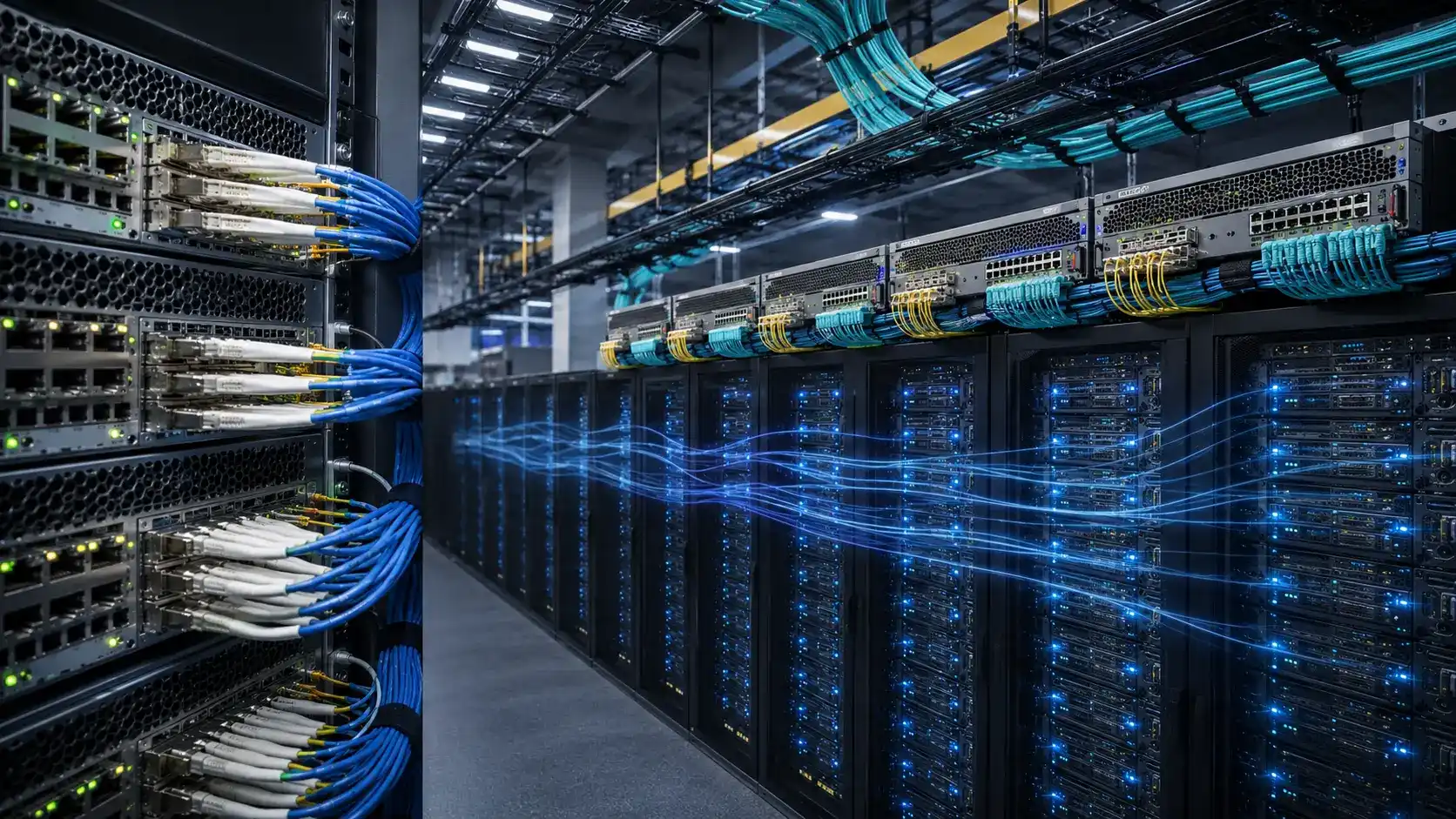
A 100G fabric produces more than bandwidth - it produces heat, airflow load, and cable density. Power budgeting should cover switch chassis and fans, QSFP28 optical modules (and DAC or AOC where used), redundant supplies, rack-level capacity, and growth margin. Cooling should account for hot- and cold-aisle layout, consistent front-to-back or back-to-front airflow, blanking panels, cable obstruction, ambient temperature, and module-temperature monitoring, because a spine packed with optics is a real thermal load.
Cabling scales fast: 16 leaves to 4 spines is already 64 leaf-to-spine links, each of which must be labeled, routed, tested, and documented. A full-mesh fabric is far easier to build and maintain with pre-terminated MPO/MTP trunk cabling than with field-terminated fiber. Teams should also settle connector and polarity conventions up front; the practical differences between MTP and MPO are worth confirming before you order. Sloppy documentation costs nothing on day one and a great deal during the first outage.
Designing for a 400G Upgrade
Design the fabric with a realistic upgrade path. You do not need 400G everywhere on day one, but you should avoid choices that make the move painful later. Start thinking about 400G readiness when spine uplinks are already heavily loaded, when adding more 100G spines is getting awkward, when ECMP path counts are nearing platform limits, or when AI, storage, or east-west growth is accelerating.
The usual strategy is to upgrade the spine first: leaves keep their 100G uplinks while a higher-capacity spine - using ports such as QSFP-DD - adds headroom, often with 400G ports breaking out into 4x100G back toward the existing leaves. The broader trajectory is set by the industry: the Ethernet Alliance roadmap now runs through 400G, 800G, and beyond, largely driven by AI. When you evaluate switches, check that the platform supports the speeds, optics, breakout modes, and software features a phased upgrade will need.
When a 100G Spine-Leaf Design Is Not the Right Choice
This design is not universal, and a few cases call for something else. A handful of servers in one or two racks rarely justify a full spine-leaf build, where a pair of redundant switches is simpler and cheaper. Very large AI training clusters may push past what a 100G access and 100G spine fabric handles well, landing on 400G or 800G fabrics - or even a dedicated InfiniBand network - from the start. And if nearly all traffic is north-south to a gateway rather than east-west between racks, the east-west advantages of spine-leaf matter less, so the topology should be justified on growth and operational grounds rather than assumed. Match the architecture to the traffic and the scale, not the other way around.
Common 100G Spine-Leaf Design Mistakes
- Counting QSFP28 ports twice. A port is either a 4x25G breakout or a 100G uplink, never both. Give every port one role.
- Choosing optics by maximum reach. Longer reach adds cost and power; match optics to the actual fiber distance and type.
- Ignoring N-1. Check the ratio during normal operation and after losing a spine.
- Forgetting optical power and heat. A spine full of QSFP28 modules is a genuine thermal load, so include optics in the power and cooling math.
- Treating cabling as an afterthought. Routing, labeling, polarity, and documentation belong in the design, not the install.
- Designing only for today's server speed. If 25G access will shift to 100G, leave room for native 100G or a 400G spine.
FAQ
Q: What is the best oversubscription ratio for a 100G spine-leaf network?
A: There is no single best ratio. For general compute, 2:1 or 3:1 is often practical. For storage, AI, HPC, or RDMA workloads, use 1:1 or a lower-oversubscription design wherever possible, and validate against measured traffic.
Q: Should I use QSFP28 SR4 or CWDM4 for leaf-to-spine links?
A: Use SR4 for short multimode runs where MPO/MTP cabling is available. Use CWDM4 or a similar single-mode optic when the distance is longer or when a duplex LC single-mode plant is preferred, up to about 2 km.
Q: Can QSFP28 break out into 4x25G?
A: Yes, many QSFP28 platforms support 4x25G breakout, but support depends on the switch model, port group, operating system, and cable type. Always check the switch compatibility matrix before designing around breakout.
Q: Is 100G spine-leaf still worth it now that 400G exists?
A: Yes, for most enterprise and cloud environments with 25G or 100G server access. 400G earns its higher cost when uplink capacity, AI traffic, or large-scale east-west bandwidth justify it.
Q: How many spine switches do I need?
A: At least two for redundancy. Larger fabrics often use four or more for better ECMP distribution and more uplink capacity. The right number depends on leaf count, uplink speed, oversubscription target, and platform limits.
Q: What is the single most common design mistake?
A: Port miscounting. Teams plan uplinks first and later discover that breakout cables consumed the QSFP28 ports they expected to use for the spine. Assign breakout ports before finalizing uplink capacity.
Conclusion
A good 100G spine-leaf design is the sum of decisions made before the hardware arrives: define the workload, count ports correctly, calculate oversubscription under both normal and failure conditions, pick optics by distance, plan breakout deliberately, budget for power and cooling, and leave room for 400G. For most enterprise data centers, 25G access with 100G QSFP28 uplinks remains a strong balance of performance, cost, and scale, while storage, AI, and HPC simply call for lower oversubscription and tighter validation. The reliable approach does not change: design from the server outward, prove the math under normal and N-1 conditions, and document every link before deployment.