AI cluster network design is the process of sizing GPU server NICs, leaf-spine bandwidth, oversubscription ratio, RoCE settings, optics and cabling so distributed training traffic remains predictable as the cluster scales. Get any of these wrong and the network - not the GPU - becomes the bottleneck.
Why AI Cluster Networking Is Different
In a traditional enterprise data center, the network handles a mix of north-south user traffic, storage access, virtualization and management. East-west traffic exists but is rarely the dominant load. In an AI cluster, the situation flips. GPU servers running distributed training exchange gradients and synchronize parameters during every step of the job. This communication is part of the computation, not a side effect of it.
If a $30,000 GPU spends 30% of its time waiting on the network during all-reduce operations, the cluster effectively pays for 30% of its compute capacity to sit idle. That is the economic reason AI networking gets so much attention.
Three workload characteristics drive the design:
- Bursty east-west traffic. Collective communication operations like all-reduce, all-gather and reduce-scatter produce synchronized bursts across many nodes simultaneously.
- Tail-latency sensitivity. A single slow node delays the entire training step. Predictable latency matters more than average latency.
- Scale-out growth. Clusters that start at 32 GPUs often grow to 256 or 1,024 within 18 months. The fabric must scale without redesign.
Why Spine-Leaf Fits AI Clusters
Spine-leaf is the standard fabric for hyperscale data centers because it gives every server-to-server path the same hop count and the same theoretical bandwidth. For AI workloads, this uniformity directly translates into more predictable training step times.
In a spine-leaf topology, GPU servers connect to leaf switches, and each leaf connects to every spine. Any GPU-to-GPU communication crosses exactly one leaf, one spine, and one more leaf. There are no aggregation layers introducing variable latency or chokepoints.

Predictable Latency
Equal-cost multi-path (ECMP) routing spreads flows across spine switches. When configured correctly with adaptive routing or dynamic load balancing, this prevents the hash collisions that cause some flows to be much slower than others - a known problem in static ECMP fabrics carrying few but large flows, which is exactly what AI training generates.
High Bisection Bandwidth
Bisection bandwidth is the throughput available between any two equal halves of the cluster. AI training benefits from non-blocking or near-non-blocking designs where the leaf-to-spine uplink capacity equals or nearly equals the downlink capacity facing the servers. The IETF defines and discusses these concepts in RFC 7938, which covers BGP-routed Clos fabrics widely used in large-scale data centers.
Easier Scale-Out
Add more leaves to add more servers. Add more spines to add more bisection bandwidth. For clusters beyond a few thousand GPUs, a super-spine (5-stage Clos) or rail-optimized topology extends the same principle one layer further.
Core Components of an AI Cluster Network
GPU Servers and NICs
The NIC is where the fabric meets the host. In AI clusters, NIC selection drives everything downstream - switch port speed, optics choice, and cabling density.
Selection criteria for AI workloads:
- Port speed: 200G, 400G or 800G per port. Match to GPU generation and PCIe bandwidth.
- PCIe generation: A 400G NIC needs PCIe Gen5 x16 to avoid host-side throttling. PCIe Gen4 x16 caps at ~256 Gbps usable.
- RDMA and RoCEv2 support: Required for kernel-bypass GPU communication libraries like NCCL.
- GPUDirect RDMA: Allows direct GPU-to-NIC DMA, removing host memory copies.
- Multi-rail capability: Many AI servers use 4 or 8 NICs per node, one per GPU pair, for rail-optimized topologies.
A typical 8-GPU server today uses either 4× 400G NICs (one per two GPUs) or 8× 400G NICs (one per GPU) depending on workload and budget. Reference architectures from NVIDIA Networking documentation cover the design tradeoffs in detail.
Leaf and Spine Switches
Switch selection criteria for AI fabrics differ from enterprise selection. Buffer size, congestion control behavior and telemetry matter more than feature breadth.
- Per-port speed and radix: A 51.2 Tbps switch ASIC delivers 64× 800G ports or 128× 400G ports. Radix determines how flat the fabric can be.
- Buffer architecture: Deep buffers absorb incast bursts but add latency. Shallow buffers reduce latency but require precise congestion control.
- RoCE feature set: ECN marking, PFC, DCQCN or equivalent congestion control, and proper handling of priority queues end-to-end.
- Telemetry: Inband network telemetry (INT), per-queue depth reporting, and microsecond-resolution counters for ECN marks and PFC pauses.
Optics, DAC and AOC Cabling
At 400G and 800G, the cabling plant becomes a real engineering problem. Form factors, link budgets and breakout configurations all need early planning.
- DAC (Direct Attach Copper): Up to ~3 meters for 400G, lowest cost and lowest power. Heavy and bulky at scale.
- AOC (Active Optical Cable): Up to ~30 meters, thinner than DAC, but fixed-length and consumes optics power on both ends.
- Pluggable optics: Required beyond AOC distance. QSFP-DD and OSFP form factors dominate 400G/800G. MPO/MTP fiber assemblies handle the parallel-fiber connections.
For inter-rack links and structured cabling at 400G/800G, parallel optics over MPO terminations are now standard. The choice between trunk cables and breakout assemblies depends on your switch port allocation - see our MPO breakout cable guide for the practical selection logic, and the broader MPO trunk vs breakout comparison when planning leaf-to-spine runs.
RoCE and Lossless Ethernet in AI Fabrics
RoCEv2 (RDMA over Converged Ethernet v2) is the dominant Ethernet transport for AI workloads. It lets NICs move data directly between GPU memory regions without kernel involvement on either end. NCCL, the GPU communication library underlying nearly all distributed training frameworks, uses RoCEv2 when InfiniBand is not available.
RoCE works well when configured correctly. It fails ugly when configured incorrectly. The InfiniBand Trade Association publishes the RoCE specifications, and most NIC and switch vendors publish detailed configuration guides that should be followed end-to-end.

Why Lossless Behavior Matters
RDMA was designed assuming a lossless transport. When packets drop, RDMA recovery is expensive - go-back-N retransmission can stall a training step for milliseconds, which is enormous relative to the microsecond-scale RDMA budget.
To approximate lossless behavior on Ethernet, the fabric uses two mechanisms working together:
- PFC (Priority Flow Control, IEEE 802.1Qbb): A switch pauses incoming traffic on a specific priority queue when its buffer fills. This is a last-resort mechanism.
- ECN (Explicit Congestion Notification, RFC 3168): Switches mark packets when queues approach a threshold. The NIC reduces its sending rate before buffers actually fill, ideally avoiding PFC entirely.
The goal is for ECN to do almost all the congestion management, with PFC as a safety net. If you see frequent PFC pauses in steady-state traffic, your ECN thresholds are wrong or your fabric is undersized.
Common RoCE Deployment Failures
| Problem | Symptom | How to Check | Fix |
|---|---|---|---|
| MTU mismatch end-to-end | Fragmentation, RDMA retries, throughput collapse | Compare NIC and switch MTU; run ping with DF bit set at MTU size | Set jumbo MTU (typically 9000 or 9216) consistently across NICs and every switch |
| PFC priority misalignment | PFC frames generated but ignored; backpressure not propagated | Check PFC priority configured on NIC vs. switch ingress queue mapping | Align DSCP-to-priority mapping on all hops |
| Wrong ECN thresholds | Either no ECN marks (congestion until PFC fires) or constant marks (throughput suppressed) | Monitor per-queue ECN-marked packet counters under realistic load | Tune Kmin/Kmax thresholds; default values rarely fit AI traffic profiles |
| Mixed traffic on same priority | Storage or management bursts disrupt training | Check DSCP markings of each traffic class at NIC and switch | Assign separate priority queues for compute, storage and management |
| Buffer exhaustion from incast | Random packet drops during all-reduce | Per-queue buffer occupancy telemetry during collective operations | Increase buffer allocation for compute priority; tune adaptive routing |
How to Design an AI Cluster Network: A Working Framework
This is the section most "AI networking" articles skip. The seven steps below give you concrete inputs and outputs at each stage.
Step 1: Define Workload and Scale
Inputs: Workload type (pretraining, fine-tuning, inference, mixed), target GPU count today, target GPU count in 18 months, model size range.
Output: A workload profile that informs NIC speed and oversubscription tolerance. Large pretraining of frontier models demands non-blocking 400G+ fabrics. Fine-tuning workloads can tolerate 2:1 oversubscription. Inference clusters often need lower bandwidth but lower tail latency.
Step 2: Choose NIC Speed and Count per Server
Decision logic:
- Pretraining of large models, 8-GPU servers → 4–8× 400G NICs per server, or 4× 800G
- Mid-scale training, 8-GPU servers → 2–4× 400G NICs per server
- Inference serving → 1–2× 200G or 400G NICs per server, depending on model parallelism
Verify PCIe bandwidth on the host. A single 400G port requires PCIe Gen5 x16 to run at line rate; doubling to 800G requires Gen6 or splitting across two slots.
Step 3: Size the Leaf Layer
Worked example - 32-node cluster, 8 GPUs per node, 4× 400G NICs per node:
- Total server-facing ports needed: 32 × 4 = 128 ports at 400G
- Downlink bandwidth per node: 4 × 400 = 1.6 Tbps
- Total cluster downlink bandwidth: 32 × 1.6 = 51.2 Tbps
Using a 64-port 400G leaf switch (25.6 Tbps total capacity), each leaf can connect 32 server ports and use the remaining 32 ports as uplinks. With 4 leaves, you cover all 128 server ports. Each leaf contributes 32 × 400G = 12.8 Tbps of uplink toward the spine.

Step 4: Size the Spine Layer
For a non-blocking (1:1) design, total uplink capacity must equal total downlink capacity. From Step 3:
- Total leaf uplink required: 4 leaves × 12.8 Tbps = 51.2 Tbps
- If each spine has 32× 400G ports = 12.8 Tbps, you need 4 spines
- Each leaf connects to all 4 spines using 8 uplinks per spine (8 × 400G × 4 = 12.8 Tbps per leaf - matches)
If using 64-port 400G spine switches, each spine has spare capacity to grow the cluster, useful for the 18-month plan from Step 1.
Step 5: Set the Oversubscription Ratio
| Workload | Recommended Ratio | Rationale |
|---|---|---|
| Large-model pretraining | 1:1 (non-blocking) | All-reduce dominates; any congestion compounds across thousands of steps |
| Fine-tuning / mid-scale training | 1.5:1 to 2:1 | Smaller collective sizes; cost savings outweigh modest slowdown |
| Inference / RAG serving | 2:1 to 4:1 | Mostly independent requests; bandwidth bursts are smaller and less synchronized |
| Mixed research cluster | 1.5:1 | Compromise between cost and unpredictable workload mix |
Step 6: Separate Compute, Storage and Management Traffic
Three options, in order of increasing isolation:
- Shared fabric with QoS classes: Compute, storage and management on separate DSCP priorities. Lowest cost; requires careful QoS configuration.
- Logically separated VLANs/VRFs: Same hardware, separate control planes. Useful for multi-tenant clusters.
- Physically separate fabrics: Dedicated NICs, switches and cabling for compute vs. storage. Highest cost; common in frontier-model clusters where any contention is unacceptable.
Storage traffic for AI is itself heavy - checkpoint writes for a large model can move hundreds of gigabytes in short bursts. Plan for it explicitly. A high-density structured cabling plant using MPO/MTP trunk cables simplifies running parallel fabrics in the same physical infrastructure.
Step 7: Validate Before Production
Network-level tests catch some problems. Workload-level tests catch the rest.
- Bandwidth: iperf3 or ib_send_bw between every node pair; should reach 90%+ of NIC line rate.
- Latency: ib_read_lat or similar; check distribution, not just average. P99.9 matters more than mean.
- Packet loss: Run 24-hour soak test under load; any non-zero loss in RoCE traffic class is a problem.
- ECN marking behavior: Verify marks appear before PFC fires; if PFC pauses are frequent in steady state, retune.
- Collective communication: Run NCCL tests (all_reduce_perf, all_gather_perf) at the full cluster size. Compare against vendor reference numbers.
- Job-level test: Run a representative training job for 4–6 hours. Watch GPU utilization - sustained values below 50% on a properly-sized model usually indicate a network problem.
Traditional Data Center Network vs AI Spine-Leaf Fabric
| Area | Traditional DC Network | AI Spine-Leaf Fabric |
|---|---|---|
| Dominant traffic | Mixed north-south and east-west | Heavy GPU-to-GPU east-west, bursty |
| Latency tolerance | Milliseconds acceptable | Microseconds matter; tail latency critical |
| Oversubscription | 4:1 to 8:1 common | 1:1 to 2:1 for training fabrics |
| Transport | TCP/IP dominant | RoCEv2 or InfiniBand |
| NIC role | Standard connectivity | Performance-critical, often multi-rail |
| Buffer requirements | Application-dependent | Tuned for incast burst absorption |
| Validation | Application response time | Per-flow telemetry + collective benchmarks |
Ethernet RoCE vs InfiniBand: Quick Decision Guide
The question comes up in nearly every AI cluster project. Both work. The choice usually comes down to operational fit, not pure performance.
- Choose InfiniBand if: Your team already operates InfiniBand fabrics, you want the simplest path to lossless transport, or you're buying a fully-integrated vendor reference architecture.
- Choose Ethernet RoCE if: Your operations team is Ethernet-native, you want multi-vendor switch options, you need to integrate the AI fabric with existing data center networks, or you anticipate scaling beyond what current InfiniBand topologies support cleanly.
The Ultra Ethernet Consortium, formed in 2023, is actively working on standardizing Ethernet enhancements specifically for AI workloads. For most new clusters in 2026, Ethernet RoCE is a defensible default unless there's a specific reason to choose otherwise.
Common Mistakes to Avoid
Upgrading Switches Without Checking NICs
An 800G switch fabric does nothing for you if your NICs run at 400G or your host PCIe runs out of bandwidth. Design the host side first, then the switch side. PCIe Gen5 x16 limits a single port to about 504 Gbps real-world throughput - comfortable for 400G, marginal for 800G.
Optimizing Port Speed but Ignoring Cabling Density
At 64-port 400G leaves, the cabling under each switch can become physically unmanageable without planning. Use breakout cables where appropriate, route fibers through structured pathways, and standardize on connector types. Connector quality and termination matter at high speeds - our fiber optic connector types guide covers the tradeoffs between LC, MPO and emerging high-density form factors.
Treating RoCE as Plug-and-Play
The biggest design mistake in real AI clusters is not picking the wrong switch - it is underestimating how much end-to-end RoCE configuration work is required. Budget time for tuning ECN thresholds, PFC priorities and MTU consistency. Plan a dedicated validation phase before any production workload runs.
Mixing All Traffic on One Fabric Without QoS
Storage replication, monitoring agents and management traffic can wreck training step times if they share buffers with compute traffic. Either separate them physically or enforce strict QoS classes with separate priorities and ECN configuration.
Building for Today's Cluster Only
Most AI clusters grow 4–8× within two years of initial deployment. Choose switch radix and spine capacity that allows non-disruptive expansion. Pulling cables in a live AI data center is expensive; planning conduit and patch capacity at deployment time is cheap.
When to Step Up from 400G to 800G
800G NICs and switches are available but more expensive per port. Consider stepping up when:
- Per-GPU bandwidth needs exceed what 400G can provide - for example, H100 and newer GPUs with NVLink 5 expect higher external bandwidth
- NCCL all-reduce times scale poorly with cluster size, indicating network saturation
- Cable density at 400G is becoming physically unmanageable - fewer 800G ports can replace more 400G ports
- The next GPU generation in your roadmap is expected to need it within the cluster's depreciation window
- You're building a frontier-model training cluster where any compute idle time costs significantly more than the optics upgrade
For most production clusters in 2026, 400G remains the right balance of cost, ecosystem maturity, and capability. 800G makes sense at the high end and as a forward investment for clusters being built today and expected to run for 4–5 years.
FAQ
Q: What is the best network architecture for AI clusters?
A: Spine-leaf Clos topology is the standard choice. For clusters above ~1,000 GPUs, extend to a 5-stage Clos (super-spine) or rail-optimized topology. The architecture itself is well-understood; the harder problems are bandwidth sizing, RoCE configuration and validation.
Q: What oversubscription ratio is acceptable for AI training?
A: For large-model pretraining, aim for 1:1 (non-blocking). For fine-tuning and mid-scale training, 1.5:1 to 2:1 is workable. For inference serving, 2:1 to 4:1 is acceptable. Higher ratios save money but reduce scaling efficiency, and the breakeven point depends on how communication-bound your workloads are.
Q: Is RoCE required for AI clusters?
A: RoCEv2 or InfiniBand is required for any cluster running NCCL-based distributed training at scale. Plain TCP/IP cannot deliver the latency and CPU efficiency needed. Between RoCEv2 and InfiniBand, choose based on operational fit and ecosystem rather than pure performance.
Q: How many NICs does a GPU server need?
A: For an 8-GPU server, common configurations are 4× 400G (one NIC per two GPUs) or 8× 400G (one NIC per GPU, rail-optimized). Inference servers may use 1–2 NICs. The decision depends on workload, GPU generation, PCIe topology and budget.
Q: Do AI clusters need separate storage and compute fabrics?
A: Small clusters can share a fabric with proper QoS class separation. Mid-size and large clusters often benefit from physically separated fabrics - compute on RoCE Ethernet or InfiniBand, storage on a dedicated Ethernet fabric. Frontier-model clusters typically separate physically because any cross-traffic interference is unacceptable.
Q: Is Ethernet better than InfiniBand for AI workloads?
A: Neither is universally better. InfiniBand has a longer track record in HPC and offers very mature lossless behavior. Ethernet RoCEv2 has broader vendor diversity, integrates with existing data center networks, and benefits from active development in the Ultra Ethernet Consortium. Operational team familiarity is often the deciding factor.
Q: What does a non-blocking AI network actually mean?
A: It means total leaf-to-spine uplink capacity equals total leaf-to-server downlink capacity, so the fabric can sustain any communication pattern between any pair of nodes at full line rate. In practice, true non-blocking is expensive; many production fabrics are "near non-blocking" at 1.1:1 or 1.2:1 and still perform well.
Q: What testing reveals real RoCE configuration problems?
A: NCCL benchmark suites (all_reduce_perf, all_gather_perf) run at full cluster scale will surface most real problems. A pure ib_send_bw test between two nodes can pass while a 32-node all-reduce performs poorly because of incast or PFC issues. Always validate at the scale you plan to run.
Conclusion
The strongest AI cluster network is not the one with the fastest switches. It is the one where NIC choice, leaf/spine sizing, oversubscription, RoCE configuration, traffic separation and physical cabling all support each other and the workload they were chosen for.
Start from the workload and the 18-month growth plan. Calculate bandwidth needs at each layer using real numbers, not just rules of thumb. Configure RoCE end-to-end and validate with real collective communication benchmarks. Budget for the cabling plant - at 400G and 800G, the physical layer is no longer trivial.
The cluster that keeps its GPUs busy at 95%+ utilization through every training step is the one that paid attention to all of these layers. The cluster that ships with a faster switch and a slower fabric will spend years explaining why the GPUs are idle.